10.2 — More Numpy, Plotting using Matplotlib

Copies and views of Numpy array

When manipulating arrays, their data may or may not be copied into a new array. Let’s look at different cases.

1x = np.arange(12)
2
3# Just a new name, no data is copied
4y = x
5
6print(x)  # [ 0  1  2  3  4  5  6  7  8  9 10 11]
7print(y)  # [ 0  1  2  3  4  5  6  7  8  9 10 11]
8print(x is y) # True, as they are same objects

When we index or slice a numpy array, the resulting array shares same data i.e. the result array is a view for the original array.

1x = np.arange(1, 13).reshape((3, 4))
2print(x)
3
4y = x[:, 1:3]  # x and y share same data
5print(y)
6
7y[0, 0] = 123  # Changing the shared data
8print(x)
9print(y)

Output

[[ 1  2  3  4]
 [ 5  6  7  8]
 [ 9 10 11 12]]
[[ 2  3]
 [ 6  7]
 [10 11]]
[[  1 123   3   4]
 [  5   6   7   8]
 [  9  10  11  12]]
[[123   3]
 [  6   7]
 [ 10  11]]

copy() method of a numpy array can be used to create a new array which does not share data with the original array.

1x = np.arange(1, 13).reshape((3, 4))
2print(x)
3
4y = x[:, 1:3].copy()
5print(y)
6
7y[0, 0] = 123  # Changes the copy only
8print(x)
9print(y)

Output

[[ 1  2  3  4]
 [ 5  6  7  8]
 [ 9 10 11 12]]
[[ 2  3]
 [ 6  7]
 [10 11]]
[[ 1  2  3  4]
 [ 5  6  7  8]
 [ 9 10 11 12]]
[[123   3]
 [  6   7]
 [ 10  11]]

np.array infers dtype based on types of numbers in the argument.

1import numpy as np
2
3x = np.array([10, 20, 30])
4print(x) #[10 20 30]
5print(x.dtype) # int64
6
7x = np.array([1.2, 3.14, 10.15])
8print(x) #[ 1.2   3.14 10.15]
9print(x.dtype) # float64
10
11x = np.array([10.0, 20, 30])
12print(x) #[10. 20. 30.]
13print(x.dtype) # float64

1import numpy as np
2
3# we can explicity specify what dtype we want:
4x = np.array([10, 20, 30], dtype=float)
5print(x) #[10. 20. 30.]
6print(x.dtype) # float64
7
8# float is truncated to int (not rounded)
9x = np.array([1.2, 3.14, 10.65], dtype=int)
10print(x) #[ 1  3 10]
11print(x.dtype) # int64

Different shapes for different purposes

[1.0 5.0 3.5 4.0 5.0 1.2]

One point in 6D euclidean space

[[1.0 5.0 3.5]
 [4.0 5.0 1.2]]

Two points in 3D euclidean space

[[1.0 5.0]
 [3.5 4.0]
 [5.0 1.2]]

Three points in 2D euclidean space

1import numpy as np
2
3x = np.arange(1, 13) # 1D array
4print(x)
5
6# 2D array, a 3x4 matrix
7matrix1 = x.reshape((3, 4))
8print(matrix1)
9
10# 2D array, a 2x6 matrix
11matrix2 = matrix1.reshape((2, 6))
12print(matrix2)
13
14 # 1D array
15y = matrix2.reshape((12,))
16print(y)

Output

[ 1  2  3  4  5  6  7  
  8  9 10 11 12]

[[ 1  2  3  4]
 [ 5  6  7  8]
 [ 9 10 11 12]]

[[ 1  2  3  4  5  6]
 [ 7  8  9 10 11 12]]

[ 1  2  3  4  5  6  7  
  8  9 10 11 12]

Special values — numpy.nan, numpy.inf

Numpy has special values to represent invalid or extreme values that result from numerical computation

numpy.nan (not a number)
numpy.inf (infinity)

1import numpy as np
2
3arr = np.array([-1, 0, 1, 2, 3, 4])
4
5print(np.log(arr))
6#[  nan   -inf  0.  0.69314718 1.09861229 1.38629436]

1# Any operation on np.nan results in np.nan
2print(np.nan * 10, 0 / np.nan)
3# nan nan
4
5# Some operations are allowed on np.inf
6
7print(np.inf, -np.inf)
8# inf -inf
9
10print(0 / np.inf, 1 / np.inf)
11# 0.0 0.0
12
13print(np.inf * np.inf, 100 + np.inf)
14# inf inf

Slicing 2D array

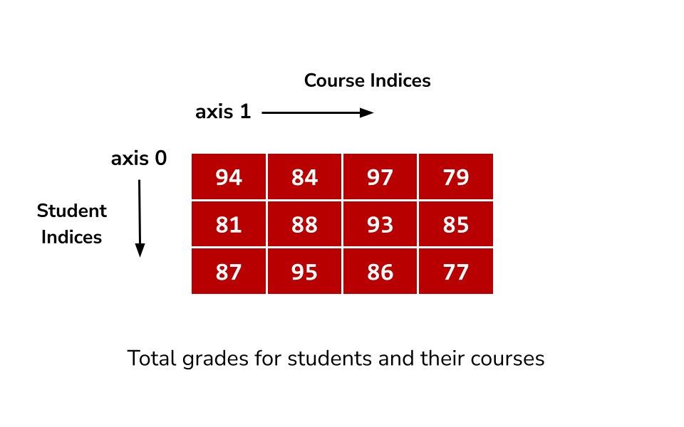
1import numpy as np
2
3grades = np.array([[94, 84, 97, 79],
4                   [81, 88, 93, 85],
5                   [87, 95, 86, 77]])
6
7print('Grades for student 1, course 2:')
8print(grades[1, 2])  # 93
9
10
11print('All grades for student 2:')
12print(grades[2, :])  # [87 95 86 77]
13
14print('All grades for course 0:')
15print(grades[:, 0])  # [94 81 87]

Assigning values using indices and slices

1import numpy as np
2
3grades = np.array([[94, 84, 97, 79],
4                   [81, 88, 93, 85],
5                   [87, 95, 86, 77]])
6
7# Setting same value to all indices in the slice
8grades[0:2, 1:3] = 100
9print(grades)
10# [[ 94 100 100  79]
11#  [ 81 100 100  85]
12#  [ 87  95  86  77]]

1import numpy as np
2
3grades = np.array([[94, 84, 97, 79],
4                   [81, 88, 93, 85],
5                   [87, 95, 86, 77]])
6
7# Setting values from array of same shape
8grades[0:2, 1:3] = np.array([[10, 20], [30, 40]])
9print(grades)
10# [[94 10 20 79]
11#  [81 30 40 85]
12#  [87 95 86 77]]

Matplotlib

Matplotlib is an extensive Python library commonly used to generate different types of plots.
To install Matplotlib: if you use Thonny, go to Tools -> Manage packages. Type matplotlib on the search bar and click “Search on PyPI”. Then click Install.
If you do not have Thonny, you can do so by typing the following commands in the terminal:
```
python -m pip install -U pip  
python -m pip install -U matplotlib  
```

matplotlib.pyplot

matplotlib.pyplot is a module in the package Matplotlib.
This is the module we’ll be using to create plots.
To use it, we first need to import it
```
import matplotlib.pyplot as plt
```
For more details: https://matplotlib.org/devdocs/api/pyplot_summary.html

Example – A Line plot

We can use the function plot to create a line plot between the points in the input sequence.

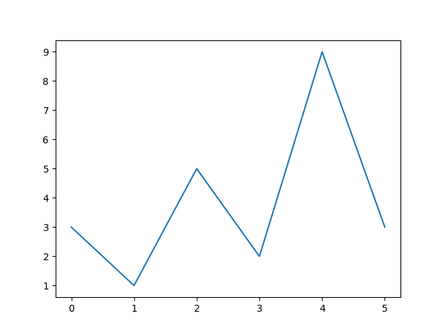
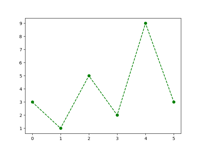
1import matplotlib.pyplot as plt
2
3some_numbers = [3, 1, 5, 2, 9, 3] 
4plt.plot(some_numbers)
5plt.show() # display figure

In the previous example:

We provided only one input to the function plot.
If we do that, then the input values are going to be considered as the y-coordinates. Their corresponding x-coordinates are the indices of the list.
In the example, we plot the following points: $(0, 3), (1, 1), (2, 5), (3, 2), (4, 9), (5, 3)$

Example - two inputs

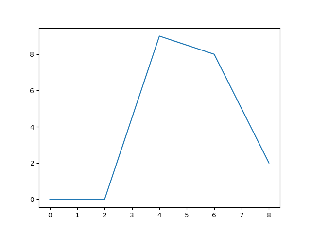
1import matplotlib.pyplot as plt
2
3x_coord = range(0, 10, 2)
4y_coord = [0, 0, 9, 8, 2]
5plt.plot(x_coord, y_coord)
6plt.show()

Example - a linear function

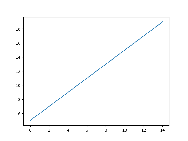
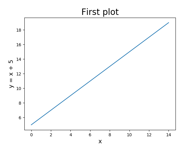
Using pyplot, we can plot the graph of the linear function $y = x + 5$ .

1import matplotlib.pyplot as plt
2
3x_coord = range(15)
4y_coord = [x + 5 for x in x_coord]
5
6plt.plot(x_coord, y_coord)
7plt.show()

Plot title and axis labels

plt.title(label): takes as argument a string and adds the title label to the figure.

plt.xlabel(label): takes as argument a string and sets the label for the x-axis.

plt.ylabel(label): takes as argument a string and sets the label for the y-axis.

We can choose the font size of the labels using the keyword argument: plt.title("First plot", fontsize=22)

1import matplotlib.pyplot as plt
2
3x_coord = range(15)
4y_coord = [x + 5 for x in x_coord]
5    
6plt.plot(x_coord, y_coord)
7
8plt.title("First plot", fontsize=20)
9plt.xlabel("x", fontsize=14)
10plt.ylabel("y = x + 5", fontsize=14)
11
12plt.show()

Colors, markers and line styles

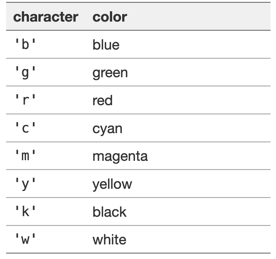
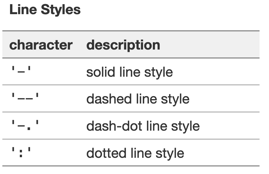
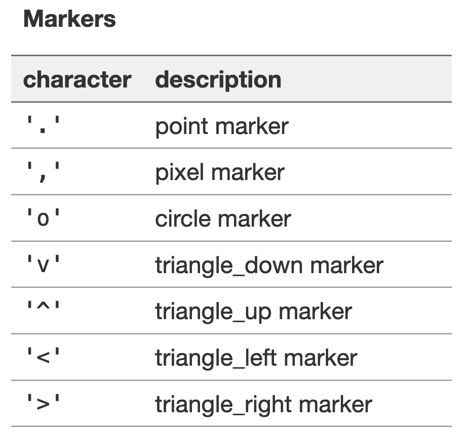
We can chose the style/color of the plots, the style/size of the markers, etc. Here is just a taste:

More info: https://matplotlib.org/stable/api/_as_gen/matplotlib.pyplot.plot.html

Using color, marker and line style

The function plot can take as arguments one or two lists (for x and y coordinates) and a format string.
The format string consists of three parts: [marker][line][color]. Each part is optional.

1import matplotlib.pyplot as plt
2
3some_numbers = [3, 1, 5, 2, 9, 3]
4
5# circle marker, dashed line, green
6plt.plot(some_numbers, "o--g") 
7plt.show() # display figure

Multiple plots in same figure

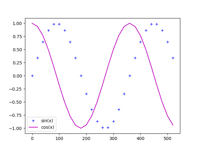
1import matplotlib.pyplot as plt
2from math import sin, cos, radians
3
4x_coord = range(0, 540, 20)
5y_sin = [sin(radians(x)) for x in x_coord]
6y_cos = [cos(radians(x)) for x in x_coord]
7    
8# + marker, blue color and use label for legend
9plt.plot(x_coord, y_sin, '+b', label="sin(x)")
10
11# magenta color and use label for legend
12plt.plot(x_coord, y_cos, 'm', label="cos(x)")
13plt.legend()  # show legend
14plt.show()

Saving a figure

plt.savefig(filename): Save the figure in a file (.jpg, .png, etc.)

1import matplotlib.pyplot as plt
2from math import sin, radians
3
4x_coord = range(0, 540, 20)
5y_sin = [sin(radians(x)) for x in x_coord]
6
7plt.plot(x_coord, y_sin, 'm')
8
9# the figure won't be displayed, but saved in y_sin.png 
10plt.savefig("myplot.png")

Bar Plots

When working with data that can be broken down into categories, it might be useful for us to use a bar plot instead.

1import matplotlib.pyplot as plt
2
3mtl_pop = [1293992, 1080545, 1015420, 1016376, 1620693, 1704694]
4years = ['1966', '1976', '1986', '1996', '2006', '2016']
5
6plt.bar(years, mtl_pop)
7
8plt.title("Population of Montreal")
9plt.show()

NumPy and Matplotlib

Matplotlib functions work with NumPy arrays as well.

1import numpy as np
2import matplotlib.pyplot as plt
3
4x_values = np.linspace(0, 8, 501)
5y_values = np.sin(x_values ** 2)  # computes sin(x^2)
6plt.plot(x_values, y_values)
7plt.show()