11.2 — Interpolation, Curve fitting, Numerical Integration

Motivation

We often want to analyze data points in the form shown below, where we have some dependent variables $y_i$ corresponding to some independent variables $x_i$ .

x_0

x_1

x_2

...

x_n

y_0

y_1

y_2

...

y_n

The goal is to find a function $f(x)$ that either
- passes through all the points exactly (interpolation)
- approximates data in a “best” possible way but not exactly (curve fitting)

Image from Kiusalaas, chap. 3.

How interpolation and curve-fitting are useful?

If we can find a function $f(x)$ that interpolates or approximates the data well,
- We can try to predict new data points $(x_k, y_k)$ .
- We can better understand the underlying process that might have generated the data.

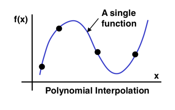
Polynomial interpolation

The simplest form of interpolation function is a polynomial function.
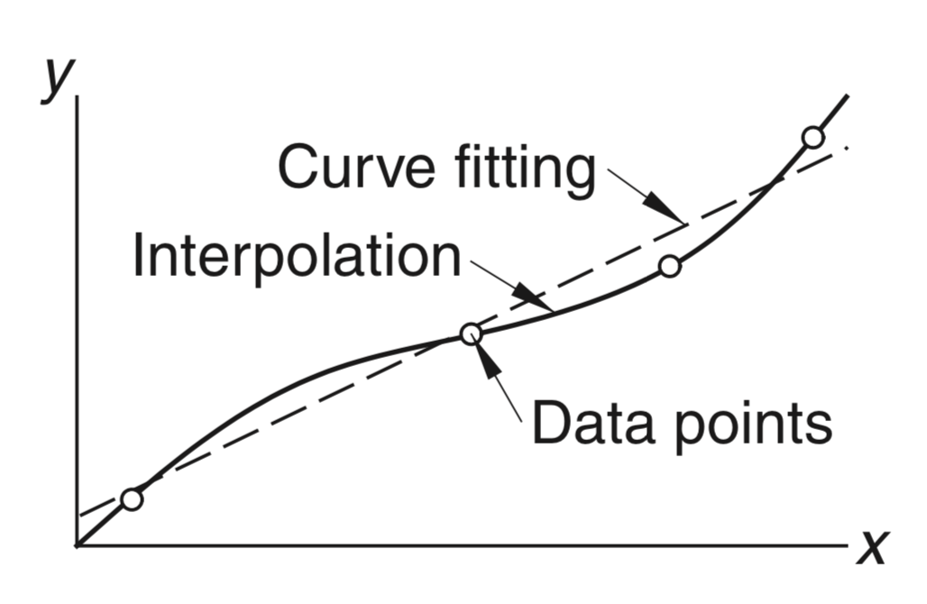
It is always possible to construct a polynomial $P(x)$ of degree $n$ that passes through $n+1$ data points.

Lagrange’s method

Suppose we have a dataset of $n+1$ points:
$(x_0, y_0), (x_1, y_1), (x_2, y_2), ..., (x_n, y_n)$
We construct an interpolation polynomial of degree $n$ , called the Lagrange polynomial, using the formula:
$P(x) = c_0(x)y_0 + c_1(x)y_1 + ... + c_n(x)y_n$
where $c_i(x)$ are called the cardinal functions.

The cardinal functions are given by:

\begin{aligned} c_i\left( x \right) &= \frac{(x-x_0)}{(x_i-x_0)} \cdots \frac{(x-x_{i-1})}{(x_i-x_{i-1})} \cdot \frac{(x-x_{i+1})}{(x_i-x_{i+1})} \cdots \frac{(x-x_{n})}{(x_i-x_{n})}\\[1em] &= \prod_{\substack{j = 0 \\[.1em] j \neq i}}^{n} \frac{(x-x_j)}{(x_i-x_j)} \end{aligned}

Numerator contains all terms except $(x - x_i)$
Denominator contains all terms except $(x_i - x_i)$

Claim: $P(x)$ passes through each data point

If $P(x)$ passes through all points $(x_i, y_i)$ , then we must have:

P(x_i) = y_i

Let’s see if this is true for the Lagrange polynomial we just found.

In the above equation for $c_i(x)$ , setting $x=x_i$ and $x=x_j$ , $i \ne j$ , we have

c_i\left( x_i \right) = \prod_{\substack{j = 0 \\[.1em] j \neq i}}^{n} \frac{(x_i-x_j)}{(x_i-x_j)} = 1

and

c_i\left( x_j \right) = \prod_{\substack{j = 0 \\[.1em] j \neq i}}^{n} \frac{(x_j-x_j)}{(x_i-x_j)} = 0\ ,\ j \neq i

Now, using the equation of $P(x)$ for $x=x_i$ :

\begin{aligned} P(x_i) &= c_0(x_i)y_0 & &+ ... + c_i(x_i)y_i & &+ ... + c_n(x_i)y_n \\ &= 0 & &+ ... + 1\cdot y_i & &+ ... + 0 \\ &= y_i \end{aligned}

Lagrange polynomial — Example

Consider the following dataset. We have $4$ data points so the degree of the Lagrange polynomial $P(x)$ will be $n=3$ .

x_i

0

10

20

30

y_i

-250

0

50

-100

We first write $4$ cardinal functions corresponding to these $4$ data points using x-values.

\begin{aligned} c_0(x) \ &= \ \frac{(x-10)}{(0-10)} \cdot \frac{(x-20)}{(0-20)} \cdot \frac{(x-30)}{(0-30)} \ = \ \frac{-1}{6000}x^3 + \frac{1}{100}x^2 - \frac{11}{60} x + 1\\ c_1(x) \ &= \ \frac{(x-0)}{(10-0)} \cdot \frac{(x-20)}{(10-20)} \cdot \frac{(x-30)}{(10-30)} \ = \ \frac{1}{2000}x^3 - \frac{1}{40}x^2 + \frac{3}{10} x\\ c_2(x) \ &= \ \frac{(x-0)}{(20-0)} \cdot \frac{(x-10)}{(20-10)} \cdot \frac{(x-30)}{(20-30)} \ = \ \frac{-1}{2000}x^3 + \frac{1}{50}x^2 - \frac{3}{20} x\\ c_3(x) \ &= \ \frac{(x-0)}{(30-0)} \cdot \frac{(x-10)}{(30-10)} \cdot \frac{(x-20)}{(30-20)} \ = \ \frac{1}{6000}x^3 - \frac{1}{200}x^2 + \frac{1}{30} x \end{aligned}

We then use these four cardinal functions along with the y-values $y_i$ in the equation of $P(x)$ :

\begin{aligned} P(x) &= c_0(x)y_0 + c_1(x)y_1 + ... + c_n(x)y_n \\ &= -x^2 + 35x -250 \end{aligned}

Download file lagrange_polynomial.py from Ed to plot these points and the interpolation function to check if it works.

Curve fitting

If data is obtained experimentally, there could be random noise present due to measurement errors.
- Interpolation would not be a good choice as it would fit all data points including noise as well.
Instead, we use curve fitting, to find a smooth curve that fits the “average” of the data points, and that is less affected by the noise or “outlier” points.

Linear regression is a simpler case of curve fitting where a straight line is found that fits a set of data points.
Unlike interpolation, the line need not pass through the points.

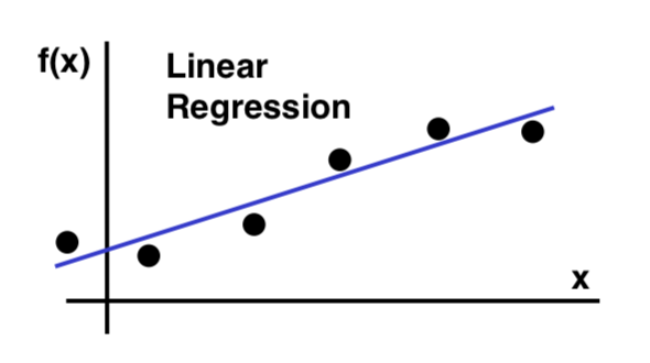
Linear regression line is given by $f(x) = ax + b$ , where $a$ is the slope of the line, and $b$ is the y-intercept.
The main task will be to find $a$ and $b$ such that the line “fits” the data points in the “best” possible way.

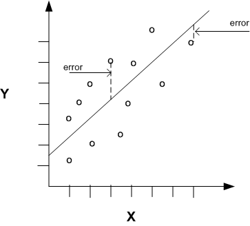
How to determine the “best” fit?

To know how good a line fits the given data points, we compute error for each data point.
Error is defined as the squared difference between the actual y-value $y_i$ and the y-value given by the regression line, $f(x_i)$ .

The total error $E$ for all data points is given by

\begin{aligned} E(a, b) &= \sum_{i=0}^{n} \left ( y_i - f\left ( x_i \right ) \right ) ^ 2 \\ &= \sum_{i=0}^{n} \left ( y_i - \left ( ax_i + b \right ) \right ) ^ 2 \end{aligned}

One way to define “best” fit:

Given all the data points $(x_i, y_i)$ , we want to find a line (i.e. find $a$ and $b$ ) such that the error $E(a, b)$ is minimized.

To find $a$ and $b$ that minimize $E(a, b)$ , we calculate the partial derivatives of $E$ with respect to $a$ and $b$ and solve for a and b when derivates are zero:

\frac{\partial E}{\partial a} = 0,\, \, \, \, \, \frac{\partial E}{\partial b} = 0

Calculating the partial derivatives

\frac{\partial E}{\partial a} = \sum_{i=0}^{n} 2 (y_i - (ax_i + b)) (-x_i)

\frac{\partial E}{\partial b} = \sum_{i=0}^{n} 2 (y_i - (ax_i + b))

Setting above derivatives to $0$ and solving for $a$ and $b$ ,

a = \frac{\sum (x_i - \bar{x}) (y_i - \bar{y}) } {\sum (x_i - \bar{x})^2 }

b = \bar{y} - a\bar{x}

where $\bar{x}$ and $\bar{y}$ are the averages of x-values and y-values of data points.

Finally, using these $a$ and $b$ , we get the desired best-fit line as $f(x)=ax+b$ . Here $a$ is slope of the line and $b$ is the y-intercept.

Download linear_regression.py from Ed, which plots data and regression line.

Interpolation examples using Numpy/SciPy

numpy_linear_interpolation.py: Piecewise linear interpolation.
cubic_spline_interpolation.py: Cubic spline interpolation — piecewise polynomial interpolation where each piece is a cubic polynomial ( $a+ b x + c x^2 + d x^3$ , $d \ne 0$ )

Definite Integral

The definite integral of a function of a single variable, $f(x)$ , between two limits $a$ and $b$ can be viewed as the area $S$ under the curve.
Numerical integration algorithms try to estimate this area

Numerical Integration

Our approach will be as follows:

Divide the region between $a$ and $b$ into $N$ segments
We then estimate the area under the curve in each segment
Finally, we sum these areas

We will consider three algorithms for estimating this area in each segment:

The Midpoint method
The Trapezoidal method
Simpson’s method

Example

We will use the following function in the interval $[0, 5]$ to compare the three algorithms:

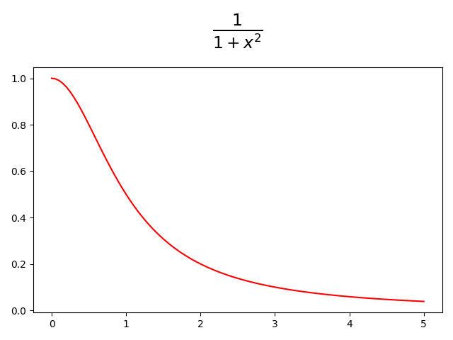
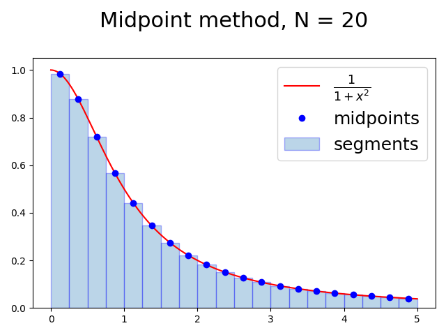
The Midpoint Method

We first divide the region from $a$ to $b$ into $N$ equal rectangular segments
The width of each segment is $\Delta x = \frac{b-a}{N}$
The endpoint of the segments are
$\small x_0 = a < x_1 < \cdots < x_{N-1} < x_{N} = b$
where
$\small x_i = a + i \cdot \Delta x, \quad i \in [0, N]$

We estimate the area under the curve in each rectangular segment using the value of $f(x)$ at the midpoint of each segment.
$\small area_k = \Delta x \cdot f(x_k + \frac{\Delta x}{2})\ ,\ k \in [0, N)$
To compute an approximation to the integral, we just have to sum these areas

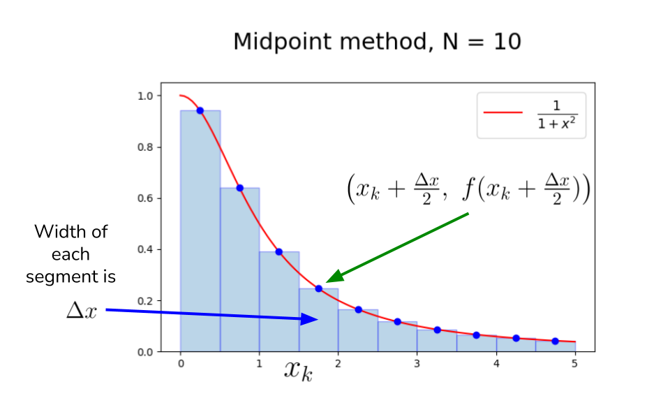
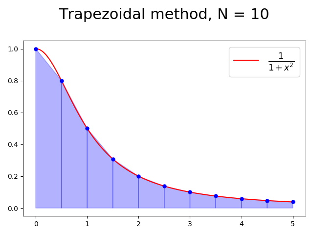
Approximation improves as the number of segments is increased.

Implementation and Error analysis of Midpoint method

1def midpoint_integrate(f, a, b, N):
2    area = 0.0
3    dx = (b - a) / N
4    x = a
5    
6    for k in range(N):
7        area += dx * f(x + dx / 2)
8        x += dx
9        
10    return area

We know the integral of the example function is given by:

\small \int_{0}^{5} \frac{1}{1+x^2} dx = arctan(5) = 1.37340076695

So, we can compute error in the result produced by our implementation midpoint_integrate.

Error of Midpoint method for different values of $N$ :

Output

    N       estimated_integral                error
-----     --------------------     ----------------
   10         1.3735434283e+00     1.4266136666e-04
   20         1.3734392602e+00     3.8493263529e-05
   40         1.3734103959e+00     9.6289197895e-06
   80         1.3734031745e+00     2.4075766312e-06
  160         1.3734013689e+00     6.0191232953e-07
  320         1.3734009174e+00     1.5047571300e-07
  640         1.3734008046e+00     3.7615273785e-08
 1280         1.3734007764e+00     9.4000809359e-09
 2560         1.3734007693e+00     2.3462840559e-09
 5120         1.3734007675e+00     5.8283222693e-10
10240         1.3734007671e+00     1.4196355203e-10

Trapezoidal Method

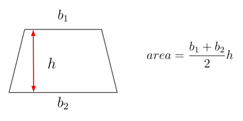
To approximate the area of each segment, use the area of trapezoid rather than the rectangle.

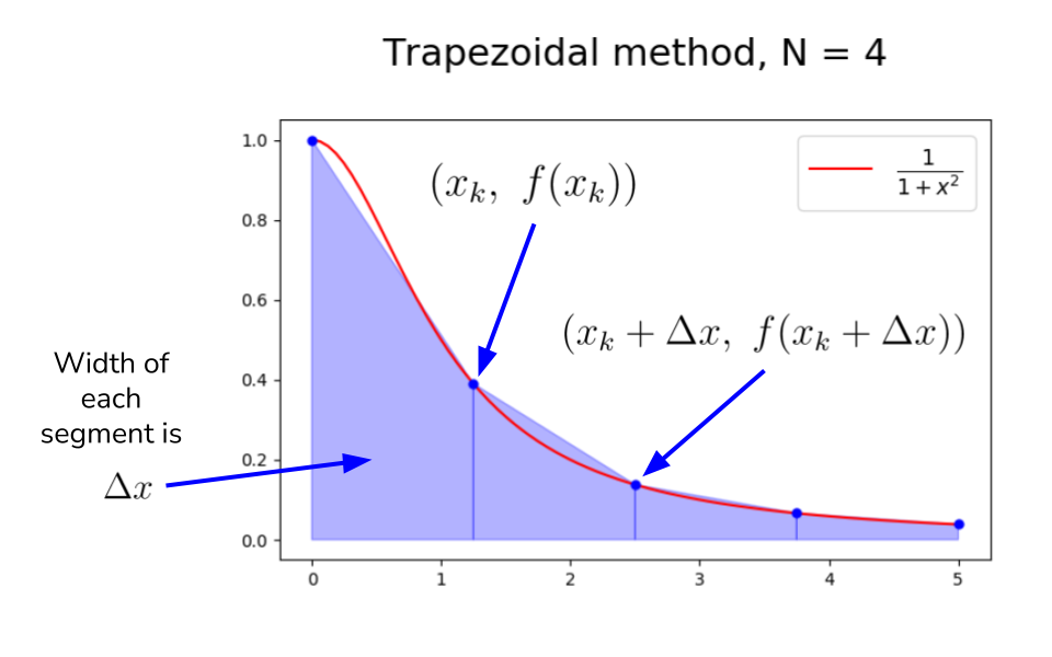
The area of each trapezoidal segment is given by

\small area_k = \frac{\Delta x}{2} \left( f(x_k) + f(x_k + \Delta x) \right)\ ,\ k \in [0, N)

Implementation and error analysis of the Trapezoidal method

area += dx * (f(x) + f(x + dx)) / 2

Output

    N       estimated_integral                error
-----     --------------------     ----------------
   10         1.3731040812e+00     2.9668571989e-04
   20         1.3733237548e+00     7.7012176612e-05
   40         1.3733815075e+00     1.9259456542e-05
   80         1.3733959517e+00     4.8152683754e-06
  160         1.3733995631e+00     1.2038458712e-06
  320         1.3734004660e+00     3.0096677106e-07
  640         1.3734006917e+00     7.5245528253e-08
 1280         1.3734007481e+00     1.8815126790e-08
 2560         1.3734007622e+00     4.7075219278e-09
 5120         1.3734007658e+00     1.1806169375e-09
10240         1.3734007667e+00     2.9889868358e-10

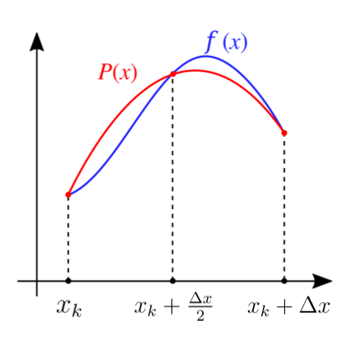
Simpson’s method

Given any three points there is a unique polynomial (parabola), called the interpolating polynomial, that passes through these points

Simpson’s method fits a parabola $P(x)$ through the curve at three points — the value of the function at the two endpoints, and at the midpoint of the interval:
$\small f(x_k),\ f(x_k + \frac{\Delta x}{2}),\ f(x_k + \Delta x)$
The area under the parabola in the interval $[x_k, x_k + \Delta x]$ is given by:
$\small \frac{\Delta x}{6} \left[f(x_k) + 4f(x_k + \frac{\Delta x}{2}) + f(x_k + \Delta x)\right]$
Adding areas of all the $N$ segments gives an approximation to the integral.

Simpson’s method generally finds a better approximation to the area under the curve in each segment than trapezoidal method which uses a line instead of parabola.
For more details on where does the formula above come from: https://en.wikipedia.org/wiki/Simpson%27s_rule

Implementation and error analysis of the Simpson’s method

area += dx * (f(x) + 4 * f(x + dx / 2) + f(x + dx)) / 6

Output

    N       estimated_integral                error
-----     --------------------     ----------------
   10         1.3733969793e+00     3.7876621872e-06
   20         1.3734007584e+00     8.5498519375e-09
   40         1.3734007664e+00     5.3898707719e-10
   80         1.3734007669e+00     3.8371528177e-11
  160         1.3734007669e+00     7.0714545330e-12
  320         1.3734007669e+00     5.1121329392e-12
  640         1.3734007669e+00     4.9893422727e-12
 1280         1.3734007669e+00     4.9857895590e-12
 2560         1.3734007669e+00     4.9855675144e-12
 5120         1.3734007669e+00     4.9795723100e-12
10240         1.3734007669e+00     4.9829029791e-12

Check implementation and example in numerical_integration.py and integration_examples.py

Accuracy of the three methods

For all the three methods we saw, as the number of subintervals $N$ approaches infinity, approximation improves and approaches actual integral.
However, the speed of improvement differs:
- Midpoint method — $error \propto \frac{1}{N^2}$
- Trapezoidal method — $error \propto \frac{1}{N^2}$
- Simpson’s method — $error \propto \frac{1}{N^4}$
Simpson’s method approaches the integral faster than other methods.

Integration using scipy.integrate

Check scipy_integrate.py file on Ed.

Motivation

How interpolation and curve-fitting are useful?

Polynomial interpolation

Lagrange’s method

Claim: P(x)P(x)P(x) passes through each data point

Lagrange polynomial — Example

Curve fitting

How to determine the “best” fit?

Calculating the partial derivatives

Interpolation examples using Numpy/SciPy

Definite Integral

Numerical Integration

Example

The Midpoint Method

Implementation and Error analysis of Midpoint method

Trapezoidal Method

Simpson’s method

Accuracy of the three methods

Integration using scipy.integrate

Claim: $P(x)$ passes through each data point