12.2 — Root Finding, Sorting algorithms

Roots of a function

A root or zero of a function $f(x)$ is a solution of the equation $f(x)=0$
Some functions can be solved in closed form i.e., their solutions can be represented in terms of functions that we know.
- $f(x) = x^2 - 1$ can be factored to $(x-1)(x+1)$ , with the solution of $f(x) = 0$ being $x = -1, 1$
For the functions that cannot be factored or represented in closed form, we must use numerical methods to find their roots.
- See this post for a discussion on “closed form”.

In general, finding roots numerically involves a procedure which generates a sequence of approximations $x_1, x_2, ..., x_n$ until we obtain a value close to the actual root.
Note that we will focus on finding the real roots to functions, not the complex roots

Single and double roots

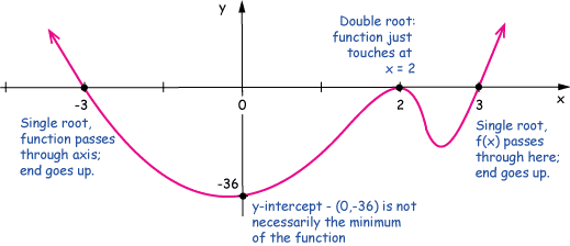
The equation $f(x)=0$ has a single root for each x-intercept i.e. each time the function $f(x)$ crosses X-axis
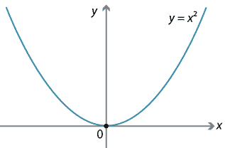
Double roots (two equal roots) occur when $f(x)$ touches but does not cross the X-axis

For example, $f(x) = x^2$ has a double root at $x=0$

Methods of finding roots

All the methods we will see require an initial estimate of the root — either a single number as an estimate or an estimated interval containing the root.
Few different ways of estimating an initial root value or interval:
- If the equation is associated with a physical problem its physical context may suggest the estimate.
- A search can be carried out for estimated root values.
- The function could be plotted (a visual procedure).

We will see the following methods in this lecture:

Bisection method
Secant method
Newton-Raphson method

Intermediate value theorem

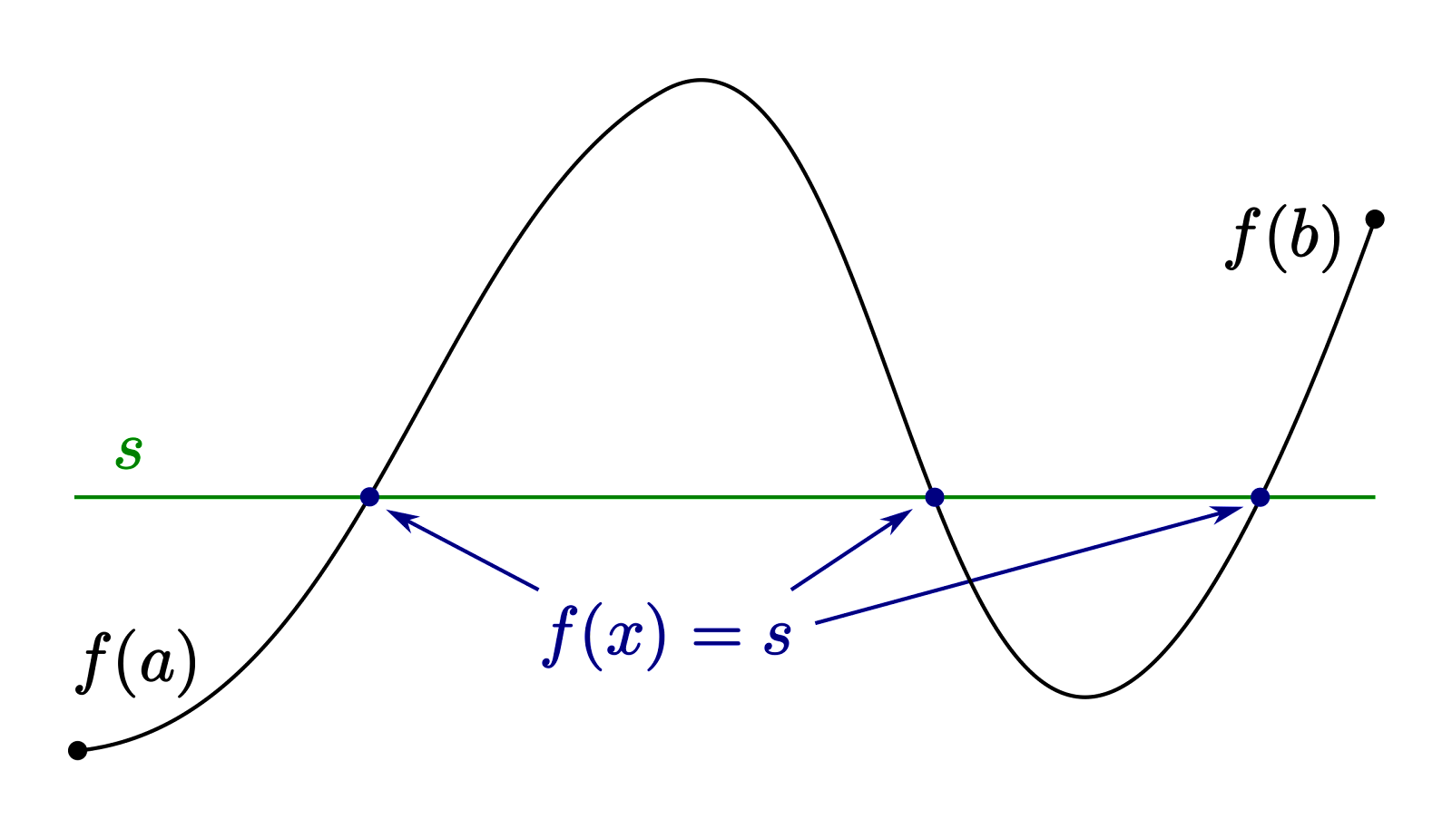
(We will assume that all functions are continuous for root finding algorithms.)

Let $f(x)$ be a continuous function on the interval $[a, b]$ and let $s$ be a number where $f(a) < s < f(b)$ , then there exists at least one $x$ with $f(x) = s$ .

We will use Intermediate value theorem in some of the root-finding methods.

The main idea is that
- If $f(a)$ and $f(b)$ have opposite signs, e.g. $f(a) < 0 < f(b)$ , then there is at least one $x$ in the interval $[a, b]$ such that $f(x) = 0$ i.e. there exists a root in $[a, b]$
Note that since a double root does not lead to a change in sign, it won’t be detectable using this method.

Checking if an interval contains a root

Given a function $f(x)$ which is continuous in the interval $[a, b]$ , if $f(a)$ and $f(b)$ have opposite signs, we have a root in $[a, b]$

1def f(x):
2    return x ** 2 - 25
3
4a1, b1 = [-4.0, 3.0]
5print('Is root in [-4.0, 3.0]?', f(a1) * f(b1) < 0)
6# False
7
8a2, b2 = [3.0, 10.0]
9print('Is root in [3.0, 10.0]?', f(a2) * f(b2) < 0)
10# True

Example

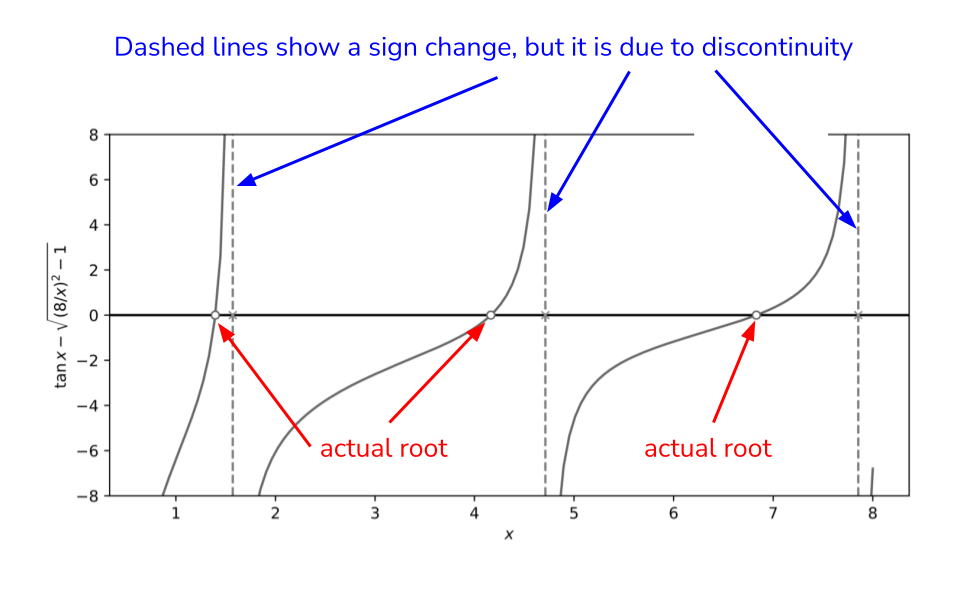
In the previous graph,

Since we have $tan$ function, which is not continuous, there are sign changes at discontinuities, e.g. in interval $[1, 2]$ .
So the theorem doesn’t work here and we can’t use the root finding methods in the interval $[1, 2]$ .
But we can find root in the interval $[6, 7]$ .

Bisection method

It is the simplest root finding algorithm which can be applied to any continuous function $f(x)$ on an interval $[a, b]$ where a root exists i.e. $f(a)$ and $f(b)$ have different signs.
Therefore, the method relies on Intermediate value theorem.
The general idea is to repeat the following
- Divide the interval in two subintervals, one of which must contain the root.
- Select the subinterval $[a_n, b_n]$ where $f(x)$ changes sign i.e. $f(a_n)·f(b_n) < 0$

Algorithm

Choose an interval $[a_0, b_0]$ where sign of $f(x)$ changes i.e. $f(a_0) \cdot f(b_0) < 0$
Compute $f(m_0)$ for the midpoint $m_0 = \frac{a_0 + b_0}{2}$
Determine the next subinterval $[a_1, b_1]$ as follows:
- If $f(a_0) \cdot f(m_0) < 0$ , then $[a_1, b_1] = [a_0, m_0]$
- If $f(m_0) \cdot f(b_0) < 0$ , then $[a_1, b_1] = [m_0, b_0]$
Repeat steps (2) and (3) until the interval $[a_n, b_n]$ is small enough, i.e. its size is less than some value $\epsilon$
Return the midpoint value $m_n = \frac{a_n + b_n}{2}$

To visualize this algorithm download visualize_bisection.py from Ed and run it.

Python implementation

Check bisection function in rootfinding.py file.

Example

f(x) = x^4 - 6.4x^3 + 6.45x^2 + 20.538x - 31.752

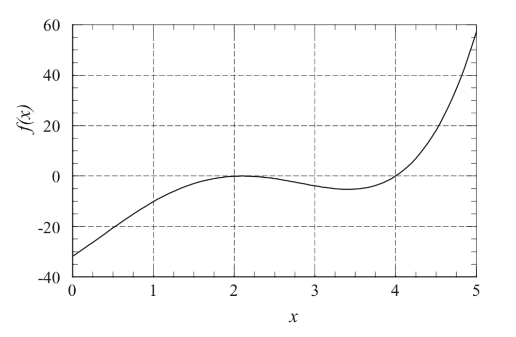
There is a double root at $x=2$ and a single root at $x=4$ .

Check Bisection method example in rootfinding_example.py file.

Secant Method

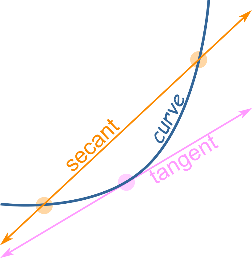
A secant line is a straight line joining at least two points on a function.

The secant method is very similar to the bisection method.
Instead of choosing the midpoint, the secant method divides each interval $[a, b]$ by the x-intercept of the secant line connecting the endpoints $(a, f(a))$ and $(b, f(b))$ .
However, unlike Bisection method, Secant method does not require that a root be present in the interval $[a, b]$ . So the Secant method may not converge to any number.

Formula for Secant line

Let $f(x)$ be a continuous function on a closed interval $[a, b]$ such that $f(a) \cdot f(b) < 0$
The secant line connecting the endpoints $(a, f(a))$ and $(b, f(b))$ is given by
$y = \frac{f(b) - f(a)}{b - a}(x - a) + f(a)$
By setting $y=0$ in above equation, we get the x-intercept of secant line as follows:
$x = a - f(a) \frac{b - a}{f(b) - f(a)}$

Algorithm for Secant method

Choose an interval $[a_0, b_0]$ where sign of $f(x)$ changes i.e. $f(a_0) \cdot f(b_0) < 0$ .
Compute $f(x_0)$ where $x_0$ is the x-intercept of secant line between $(a_0, f(a_0))$ and $(b_0, f(b_0))$ given by $x_0 = a_0 - f(a_0) \frac{b_0 - a_0}{f(b_0) - f(a_0)}$
Determine the next subinterval $[a_1, b_1]$ as follows:
- If $f(a_0) \cdot f(x_0) < 0$ , then $[a_1, b_1] = [a_0, x_0]$
- If $f(x_0) \cdot f(b_0) < 0$ , then $[a_1, b_1] = [x_0, b_0]$
Repeat steps (2) and (3) until the interval $[a_n, b_n]$ is small enough or some fixed number of steps have been taken.
Return the value $x_n$ , the x-intercept of $n^{th}$ subinterval.

To visualize this algorithm download visualize_secant.py from Ed and run it.

Python implementation

Check secant function in rootfinding.py file.

Check Secant method example in rootfinding_example.py file.

Newton-Raphson method

Simple, fast, and best-known method of finding roots.
It uses derivative of the function $f(x)$ i.e. tangent line.
- So, it can only be used if the function is differentiable in the given interval.
- If it is costly to compute the derivative, Newton’s method will be slow.
It doesn’t need an interval as an initial estimate, but only one estimate value $x_0$ .

We start with an approximation of the root, $x_0$ and compute successive approximations as follows:
$x_n = x_{n-1} - \frac{f(x_{n-1})}{f'(x_{n-1})}$
The above formula comes from Taylor series approximation of $f(x_n)$ given by:

$f(x_n) \approx f(x_{n-1}) + f'(x_{n-1})(x_n - x_{n-1})$
- Setting $f(x_n)$ to $0$ and solving for $x_n$ would give the above formula for $x_n$ .
This method may not converge. To prevent an infinite loop, we use a fixed number of iterations, and stop if we do not find a root.

To visualize this algorithm download visualize_newton.py from Ed and run it.

Python implementation

Check newton_raphson function in rootfinding.py file.

For Newton-Raphson we also need the first derivative of the function. For the exampl we have,

f(x) = x^4 - 6.4x^3 + 6.45x^2 + 20.538x - 31.752

f'(x) = 4 x^3 - 19.2 x^2 + 12.9 x + 20.538

Check the example in rootfinding_example.py file.

Newton-Raphson divergence examples

Although the Newton–Raphson method converges fast near the root, its global convergence characteristics are poor.

Method	Assumptions	Convergence	Can find Double roots?
Bisection	$f$ is continuous, root exists in the initial interval	Yes	No
Secant	$f$ is continuous, root need not exist in the initial interval	Not guaranteed but will converge if root is close to initial interval.	Not guaranteed.
Newton-Raphson	$f$ is continuous and differentiable	Not guaranteed, but will converge if initial estimate is close to root.	Yes but may converge slowly.

Speed of convergence (single root): Newton-Raphson > Secant > Bisection

Root-finding using Scipy

Check the file scipy_rootfinding.py.