11.1 — More Numpy, Linear algebra, Random numbers

Numpy arrays and for loop

1import numpy as np
2
3x = np.arange(1, 13)
4print(x)
5print(x.shape)
6
7for i in range(x.shape[0]):
8    x[i] = x[i] ** 2
9    
10print(x)
11print(x.shape)

Output

[ 1  2  3  4  5  6  
7  8  9 10 11 12]
(12,)
[  1   4   9  16  25  36  
49  64  81 100 121 144]
(12,)

1import numpy as np
2
3matrix = np.arange(1, 13).reshape((3, 4))
4print(matrix)
5print(matrix.shape)
6
7for i in range(matrix.shape[0]):
8    for j in range(matrix.shape[1]):
9        matrix[i, j] = matrix[i, j] ** 2
10    
11print(matrix)
12print(matrix.shape)

Output

[[ 1  2  3  4]
 [ 5  6  7  8]
 [ 9 10 11 12]]
(3, 4)
[[  1   4   9  16]
 [ 25  36  49  64]
 [ 81 100 121 144]]
(3, 4)

Comparison operation with NumPy array

When comparison operators are used with NumPy arrays, result is an array of boolean values.

1import numpy as np
2
3arr = np.array([10, 11, 12, 13, 14, 15, 16, 17])
4print(arr % 2 == 0) # produces numpy array of booleans
5# [ True False  True False  True False  True False]
6
7arr = np.array([-10, -20, 0, 24, -50, 33, 10])
8print(arr > 0)
9# [False False False  True False  True  True]

Using a list/array of booleans as index

1import numpy as np
2
3arr = np.array([10, 11, 12, 13])
4indices = [True, False, False, True]
5# For each i, select arr[i] if indices[i] is True:
6print(arr[indices])  # [10 13]
7
8arr = np.array([10, 11, 12, 13, 14, 15, 16, 17])
9print(arr[arr % 2 == 0])  # [10 12 14 16]
10
11arr = np.array([-10, -20, 0, 24, -50, 33, 10])
12print(arr[arr > 0])  # [24 33 10]

Using a list/array of integers as index

Multiple elements of a numpy array can be selected using a list or an array of indices.

1nums = np.arange(10, 100, 10)
2# [10 20 30 40 50 60 70 80 90]
3
4indices = [0, 1, 5]
5print(nums[indices]) # [10 20 60]
6
7# Output will be in same order as indices
8indices = np.array([2, 8, 5, 1])
9print(nums[indices]) # [30 90 60 20]

Indexing 2D arrays with list/array of indices:

1import numpy as np
2matrix = np.arange(1, 13).reshape((3,4))
3print(matrix)
4
5# Select rows 0 & 2
6row_indices = [0, 2]  
7print(matrix[row_indices, :])
8
9# Select columns 1 & 2
10col_indices = [1, 2]
11print(matrix[:, col_indices])
12
13# Select numbers at (0, 1) and  (2, 2)
14print(matrix[row_indices, col_indices])

Output

[[ 1  2  3  4]
 [ 5  6  7  8]
 [ 9 10 11 12]]

[[ 1  2  3  4]
 [ 9 10 11 12]]

[[ 2  3]
 [ 6  7]
 [10 11]]

[ 2 11]

Vector and Matrix operations in NumPy

1import numpy as np
2v = np.arange(10, 70, 10)  # 1D array as vector
3print(v)  #[10 20 30 40 50 60]
4
5M = np.arange(10, 100, 10).reshape((3,3))  # 2D array as matrix
6print(M)
7# [[10 20 30]
8#  [40 50 60]
9#  [70 80 90]]
10
11# ndarray.size attribute — total number of elements in ndarray
12print(v.size)  # 6
13print(M.size) # 9

Stacking new rows/columns into a matrix

Size of new row/col must match that of the matrix row/col.

1import numpy as np
2M = np.arange(1, 7).reshape((2, 3))
3print(M)
4
5v = np.array([-1, -2])
6M2 = np.column_stack([M, v])
7print(M2)
8
9w = np.array([5, 7, -1])
10M3 = np.row_stack([M, w])
11print(M3)

Output

[[1 2 3]
 [4 5 6]]
[[ 1  2  3 -1]
 [ 4  5  6 -2]]
[[ 1  2  3]
 [ 4  5  6]
 [ 5  7 -1]]

Matrix Multiplication

Interactive explanation for matrix multiplication: https://observablehq.com/@meetamit/matrix-multiplication
The @ operator performs matrix multiplication with NumPy arrays.
- np.dot can also be used to do matrix multiplication.
Recall that * operator performs element-wise multiplication.

1import numpy as np
2A = np.arange(10, 70, 10).reshape((3, 2))
3B = np.arange(10, 70, 10).reshape((2, 3))
4print(A)
5#[[10 20]
6# [30 40]
7# [50 60]]
8print(B)
9#[[10 20 30]
10# [40 50 60]]
11
12C = A @ B
13print(C)
14#[[ 900 1200 1500]
15# [1900 2600 3300]
16# [2900 4000 5100]]

1import numpy as np
2
3A = np.array([[83, 10, 39],
4              [29, 67, 81]])
5print(A @ A)
6# ValueError: matmul: Input operand 1 has a mismatch in 
7# its core dimension 0, (size 2 is different from 3)

Example

Let’s compute the following

\small 2A + AB - 3I

where given matrices A and B (I is the identity matrix). Shapes of all matrices must match.

1import numpy as np
2
3A = np.array([[1, 5], [-2, 9]])
4B = np.array([[2, 5], [1, -2]])
5I = np.eye(2) # 2x2 identity matrix
6
7result = 2 * A +  A @ B - 3 * I
8print(result)

Powers of a matrix

1import numpy as np
2from numpy.linalg import matrix_power
3
4A = np.array([[1, 5], [-2, 9]])
5
6# Cube of the matrix A
7print(A @ A @ A)
8#[[-109  405]
9# [-162  539]]
10
11# Another way, using library function:
12print(matrix_power(A, 3))

Random numbers and Monte Carlo methods

Python random module

1import random
2
3nums = [5, 4, 3, 2, 100, 1]
4
5# Randomly choose one item from mylist
6print(random.choice(nums))  # 5
7
8# Randomly choose a list of 3 items from the list
9# An element in the list is chosen only once.
10print(random.sample(nums, 3))  # [4, 5, 100]

Random numbers in NumPy

1import numpy as np
2
3# All output numbers below will change each time your run the code.
4# But shape of arrays should remain same.
5
6x = np.random.random() # a random float in [0, 1)
7print(x)  # 0.2894424639826647
8
9# array of 5 floats, each value in [0, 1)
10nums = np.random.random(5)
11print(nums)
12# [0.564407   0.36047169 0.68956636 0.11457356 0.26594372]

1import numpy as np
2
3# 3x2 matrix, each float in [0, 1)
4matrix = np.random.random((3, 2))
5print(matrix)
6# [[0.573776   0.37419411]
7#  [0.23126045 0.32425979]
8#  [0.81373111 0.33039031]]
9
10# random integer  in [1, 5)
11x = np.random.randint(1, 5)
12print(x)  # 2

1import numpy as np
2
3# random array of size 7, each integer in [1, 5)
4nums = np.random.randint(1, 5, 7)
5print(nums)  # [4 4 1 3 3 1 4]
6
7# 3x2 matrix, each integer in [1, 10)
8matrix = np.random.randint(1, 10, (3, 2))
9print(matrix)
10# [[4 7]
11#  [4 6]
12#  [3 9]]

1import numpy as np
2
3nums = [5, 4, 3, 2, 100, 1]
4# choose a single number from list
5x = np.random.choice(nums)
6print(x)  # 4
7
8# Choose 10 numbers from the list.
9# Each number is chosen independently, so numbers may repeat.
10many = np.random.choice(nums, 10)
11print(many)
12# [3 4 3 3 3 1 5 2 4 2]

Example: throwing an unbiased die

Let’s throw an unbiased six-sided die and count the number of occurrences of 4.
Unbiased or unweighted means that every integer from 1 to 6 is equally likely to roll. That is, the die is “fair”.

1import random
2
3options = [1, 2, 3, 4, 5, 6] # six faces of the die
4num_rolls = 1000
5
6num_fours = 0
7for i in range(num_rolls):
8   roll = random.choice(options)
9   if roll == 4:
10      num_fours += 1
11
12print("Frequency of 4:", num_fours / num_rolls)

Let’s do the same using NumPy:

1import numpy as np
2
3options = np.arange(1, 7) # six faces of the die
4num_rolls = 1000
5
6rolls = np.random.choice(options, num_rolls)
7freq = rolls[rolls == 4].size / num_rolls
8
9print("Frequency of 4:", freq)

Example: throwing a biased or weighted die

Let’s throw a biased, or weighted, six-sided die where we favor number 3 over others by giving it more “weight” or probability.
- Such a die would be called “unfair.”

1import numpy as np
2
3options = [1, 2, 3, 4, 5, 6]
4
5# Assign unequal weights or probabilties to each choices
6# Weights must sum to 1.0
7weights = [.1, .1, .5, .1, .1, .1 ]
8
9num_rolls = 1000
10
11rolls = np.random.choice(options, num_rolls, p=weights)
12freq = rolls[rolls == 3].size / num_rolls
13
14print("Frequency of 3:", freq)

Monte Carlo methods

A type of algorithm that uses random sampling to solve problems.
There are Monte Carlo methods for many different problems in physics, chemistry, AI and engineering.
- https://en.wikipedia.org/wiki/Monte_Carlo_method#Engineering
We will see a simple case here with a Monte Carlo method for integration.

Finding the area of a complex shape

Let’s say we have a complex shape and we want to find its area.
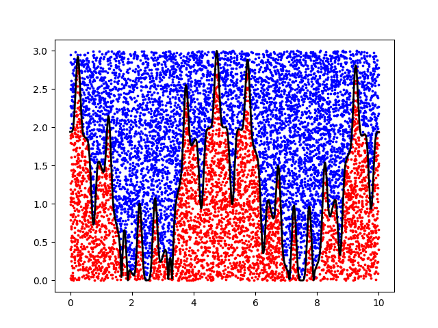
We will draw a rectangle around this shape, then sample random points inside the rectangle.
Then we can estimate the area of the inner shape by multiplying the rectangle’s area by the fraction of points that land inside the shape.

\small \textup{area}_\textup{shape} \approx \textup{area}_\textup{rectangle} * \frac{\textup{points}_\textup{inside}}{\textup{points}_\textup{inside} + \textup{points}_\textup{outside}}

Monte Carlo integration

We can use the above idea of finding area to numerically integrate a function.
For a given function $f(x)$ , we define a rectangle that bounds $f(x)$ along X-axis between $[a, b]$ and along Y-axis between $[0, c]$ , where
$\small c >= \max_{x \epsilon (a, b)} f(x)$
Then we can estimate the integral by randomly choosing points inside the rectangle, and using the formula of area from the previous slide.

Example:

Consider the following function:
$\small f(x) = \left | sin(2\pi x)^5 - 2cos(3cos( \frac{x}{\pi} )^2)^3 \right |$
We can’t integrate this analytically (i.e. representing it in terms of standard math functions).
So let’s use Monte Carlo integration instead.

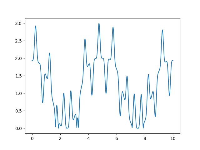
1import numpy as np
2import matplotlib.pyplot as plt
3
4
5def f(x): # x is numpy array
6    y = np.sin(2 * np.pi * x) ** 5
7    y -= 2 * np.cos(3 * np.cos(x / np.pi) ** 2) ** 3
8    return np.abs(y)
9
10
11x = np.linspace(0, 10, num=1001)
12plt.figure()
13plt.plot(x, f(x))
14plt.show()

Suppose we want to calculate the definite integral of $f(x)$ in interval $[0, 10]$
We then choose the rectangle bounds as:
- $[0, 10]$ along X-axis
- $[0, 3]$ along Y-axis because from the plot $\small 3 >= \max_{x \epsilon (0, 10)} f(x)$
Then, we compute number of points below the function f(x) in the above defined rectangle
Check montecarlo_integration.py for the implementation.

There are several methods that can perform Monte Carlo integration.
The one we’ve seen is called the rectangle method, or dart method.
It can only be used for simple functions and its accuracy is not very high.

Numpy arrays and .css-70ydf1{background-color:#d6cbc5;color:black;border-radius:3px;padding:0.1em 0.3em;font-family:Hack;font-size:0.75em;white-space:pre;}for loop

Comparison operation with NumPy array

Using a list/array of booleans as index

Using a list/array of integers as index

Vector and Matrix operations in NumPy

Stacking new rows/columns into a matrix

Matrix Multiplication

Example

Powers of a matrix

Random numbers and Monte Carlo methods

Python random module

Random numbers in NumPy

Example: throwing an unbiased die

Example: throwing a biased or weighted die

Monte Carlo methods

Finding the area of a complex shape

Monte Carlo integration

Numpy arrays and for loop